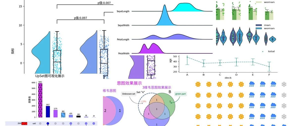
背景介绍 大家好。本公众号覆盖数据分析、可视化、大模型等多个方向实用技巧分享,欢迎大家关注,具体可查看下面文章:
如果对你有帮助,还请关注下面公众号点赞关注转发,你的支持就是我创作的最大动力~
今天给大家分享数据分析高达17种高级图表 可视化本文涉及的python库版本信息如下:
# !pip install great_tables==0.5.0
# !pip install polars==0.20.18
# !pip install mpl_font==1.1.0
# !pip install pywaffle==1.1.0
# !pip install ptitprince==0.2.7
# !pip install matplotlib_venn
# !pip install upsetplot==0.9.0
# !pip install plottable==0.1.5
# !pip install pyjanitor==0.26.0
# !pip install pynimate==1.3.0
本文目录 华夫图绘制 PyWaffle库(其官方github:https://github.com/gyli/PyWaffle)是基于matplotlib库进行二次开发。主要用于绘制华夫图(象形图),只需要一行代码即可快速绘制,其支持高达2k多种象形图标。下面是常用的案例介绍
import matplotlib.pyplot as pltfrom pywaffle import Waffle"sun" : 30 , "showers" : 16 , "snowflake" : 4 }5 ,"#FFA500" , "#4384FF" , "#C0C0C0" ],"sun" , "cloud-showers-heavy" , "snowflake" ],20 ,"solid" ,True ,f"{k} :{v} ({int(v / sum(data.values()) * 100 )} %)" for k, v in data.items()],"ncol" : len(data),"loc" : "lower left" , "bbox_to_anchor" : (-0.05 , -0.2 ),"frameon" : False ,"fontsize" : 12 ,'labelspacing' :0.2 ,}效果展示
瀑布图精美可视化 瀑布图(Waterfall Chart)是一种专门用于表现数据在一系列变化后累积效果的图表类型,它通过一连串的垂直条形来可视化数据随时间或其他顺序变量的变化过程,尤其强调从一个初始值到最终值之间每个阶段对总体数值的贡献或影响。下面是利用python绘制的瀑布图。
index = ['初始值' ,'1月份' ,'2月份' ,'3月份' ,'4月份' ,'5月份' ]10 ,-30 ,-7.5 ,-25 ,95 ,-7 ]'A' : b},index=index)'B' ] = [20 ,10 ,-40 ,30 ,20 ,-10 ]import mpl_font.noto2 ,1 , figsize=(8 ,6 ), dpi=144 )0 ]'A' ,'{:,.2f}' ,0 , net_label='最终值' ,'瀑布图可视化展示' , x_lab='月份' , y_lab='产量' 1 ]'B' ,'{:,.2f}' ,0 , net_label='最终值' ,'瀑布图可视化展示' , x_lab='月份' , y_lab='产量' ,'#4BC0E7' , red_color='#A07AED' , blue_color='#C04BE7' ,可视化展示
云雨图+显著性展示 云雨图(Raincloud plot)是一种结合了多种图形元素的统计图表,用于更全面地展示数据分布特征以及多个组别之间的比较。它通常包括以下几个组成部分:
云(Cloud) :这部分采用核密度估计(Kernel Density Estimation, KDE)来描绘数据的概率密度分布,类似于小提琴图(Violin plot),但有时可能只显示一侧或者经过修改以减少视觉混乱。
伞(Umbrella) :即箱线图(Boxplot)的部分,显示了数据的四分位数(最小值、下四分位数、中位数、上四分位数、最大值),概括了数据的基本集中趋势和离散程度。
雨(Rain) :散布在箱线图下方的点状图,展示了每个数据点的位置,有助于观察单个数据值相对于整个分布的情况。
下面是利用PtitPrince库(官方github:https://github.com/pog87/PtitPrince)来快速实现云雨图可视化
import mpl_font.notoimport matplotlib.pyplot as pltfrom ptitprince import PtitPrince as pt10 , 6 ), dpi=144 )"A" ; dx = "Category" ; ort = "v" # 显示一半小提琴"云图" "cool" , bw=.2 , linewidth=1 ,cut=0. ,scale="area" , width=.8 , inner=None ,orient=ort,x=dx,y=dy)# 显示点状图"雨图" "cool" , edgecolor="white" ,size=2 ,orient=ort,x=dx,y=dy,jitter=1 ,zorder=0 )# 显示箱型图 "black" ,orient=ort,width=.15 ,x=dx,y=dy,zorder=10 , showcaps=True ,boxprops={'facecolor' :'none' , "zorder" :10 },showfliers=True ,whiskerprops={'linewidth' :2 , "zorder" :10 },saturation=1 )# 进行单边t检验&&绘制对应的效果 'A' ].max() + 0.8 ;h= 1 ;col = 'k' 'type_A' , 'type_B' ), ('type_B' , 'type_C' ), ('type_A' , 'type_C' )]for i, (group1, group2) in enumerate(pairs):'Category' ] == i]['A' ]'Category' ] == i+1 ]['A' ]1.2 , c=col).5 , y+h+(h*i), f'p值:{p_value:.3 f} ' , ha='center' , va='bottom' , color=col)# 配置坐标轴 -11 , y+h+3 *h)-0.7 , right=3.5 )'type_A' ,'type_B' ,'type_C' ,'type_D' ],ha='right' ,rotation = 0 ,fontsize = 12 ) # 设置刻度标签 '云雨图+箱型图+显著性可视化展示' ,y=1.01 )'不同类型' )'指标' )False )"top" ].set_visible(False )"right" ].set_visible(False )可视化结果:
分组统计柱状图使用seaborn库快速实现分组统计柱状图 下面是利用seaborn库快速实现分组统计柱状图,对应的python案例如下。
import seaborn as snsimport numpy as npimport matplotlib.pyplot as pltimport matplotlibimport warnings"matplotlib:" , matplotlib.__version__)"ignore" )"titanic" )'who' ].isin(['man' ,'woman' ])].query("deck!='G'" )from pandas.api.types import CategoricalDtype'deck' ]=df['deck' ].astype( CategoricalDtype(categories=['A' ,'B' ,'C' ,'D' ,'E' ,'F' ], ordered=True ))'deck' ].unique()3 ,1 , figsize=(6 ,6.5 ),dpi=200 , )0 ]"deck" , "age" , hue="who" , errorbar=("ci" , 85 ),estimator=np.mean,'#5CBB45' ,'#DEEBB5' ],.2 ,0.5 , #设置柱状图的宽度 1 ,'v' ,) #estimator=np.mean, ci=85, "deck" ,"age" ,hue="who" ,dodge=True ,jitter=True , ax=ax,'green' ,'#5CBB45' ],size=3 ,orient='v' ,legend=False )'man' ,'woman' ],ncol=1 ,frameon=False ,loc='upper right' )'right' ].set_visible(False )'top' ].set_visible(False )'bottom' ].set_visible(False )False )1 ]"deck" ,hue="who" ,palette=['#4057A8' ,'#22AFE5' ],"age" ,dodge=True , ax=ax,orient='v' ,legend=False )"deck" ,hue="who" ,size=3 ,palette=['#40F7A8' ,'#4057A8' ],"age" ,dodge=True , ax=ax,orient='v' ,legend=False )'man' ,'woman' ],ncol=1 ,frameon=False ,loc='upper right' )'right' ].set_visible(False )'top' ].set_visible(False )'bottom' ].set_visible(False )False )20 *i for i in range(6 )])20 *i for i in range(6 )])2 ]"deck" , y="age" , orient='v' ,dodge=True ,"x" ,linestyles= "--" ,errwidth=1 ,"se" ,3 ), capsize=.2 , scale=0.5 , ax=ax,color='#43978F' ,join=True ,label='total' ) #['#43978F','#ABD0F1'] 'total' ],ncol=1 ,frameon=False ,loc='upper right' )'right' ].set_visible(False )'top' ].set_visible(False )0.1 )可视化结果:
热力图:利用biokit库绘制精美热力图 当你需要展示二维数据的整体变化趋势时,你可以使用biokit库(https://github.com/biokit/biokit)来进行可视化展示,下面是一个案例分享;
# !pip install biokit==0.5.0 for k in ['A' ,'B' ,'C' ,'D' ,'E' ,'F' ,'G' ])))'circle' , shrink=.9,lower='circle' , label_color='red' 'cool' )'crest' ,method='square' , shrink=.9 ,rotation=45)'copper' , method='text' ,)'pie' )可视化结果:
同类型不同阶段对比图:使用双系列重叠图表示 下面是一个案例展示利用双系列重叠图表示同类型不同阶段数据指标的变化情况。
from mplfonts.util.manage import use_font'Noto Sans CJK SC' )import matplotlib.pyplot as pltimport mplcyberpunkimport numpy as np'%d月' %i for i in range(1 ,13 )]45 , 63 , 49 , 45 ,53 ,45 ,67 ,64 ,73 ,84 ,64 ,55 ])25 , 93 , 29 , 85 ,63 ,25 ,47 ,84 ,43 ,94 ,34 ,25 ])# DCE9F4', '#E56F5E', '#F19685','#FFB77F', '#F6C957', '#FBE8D5'] with plt.style.context("cyberpunk" ):'Noto Sans CJK SC' )2 ,1 ,figsize=(6 ,2.5 ),dpi=200 )0 ]"产品A实际完成和预计完成情况" , fontsize=8 )4 ) for i in range(len(y1))])'#E56F5E' for _ in range(len(x))])0 ]='#F6C957' 0.4 ,)for index,value in enumerate(y1):if delta_list[index]>0 :0.01 , f'{delta_list[index]*100 :0.2 f} %' , ha='center' , va='bottom' , color='#FBE8D5' ,fontsize=6 ,)else :-0.03 , f'{delta_list[index]*100 :0.2 f} %' , ha='center' , va='top' , color='#FBE8D5' ,fontsize=6 ,)False )False )0 , linestyle='--' , color=(194 /255 ,127 /255 , 159 /255 ), linewidth=1 )'完成率' ],fontsize=6 ,ncol=2 ,loc='upper left' )#'upper right',) 1 ]'#ABD0F1' ,width=0.6 ,label='实际值' )for index,value in enumerate(y1):8 , f'{value} ' , ha='center' , va='top' , color='#E56F5E' ,fontsize=6 ,) '#43978F' ,label='预估值' )for index,value in enumerate(y2):8 , f'{value} ' , ha='center' , va='top' , color='#E56F5E' ,fontsize=6 ,) 10 *i for i in range(15 )])10 *i for i in range(15 )])False )0 ].legend([o1,o2,delta,],['实际值' ,'预估值' ,'完成率' ],fontsize=6 ,ncol=3 ,loc='upper right' )#'upper right',) 0.01 ,wspace=0.01 )输出效果图:
滑珠图: 绘制滑珠图展示不同产品2个阶段的对比 import pandas as pd'2019' :[42,21,53,16,23,10,20,65,16,34,13,25,18,25,14,26]})'Product' ] = ['A_%d' %i for i in range(16)]'2020' ] = df['2019' ].apply(lambda x:x +30+ int(10*np.random.random()) )'2020' ]= 30'white' ,edgecolor='white' )'white' )#绘制线 '2019' ], xmax=df['2020' ], color="k" , lw=1)#添加线标记 for i,v1,v2 in zip(df.index,df['2019' ],df['2020' ]):if v2>v1:"+%d" %(v2-v1),size=10,color='#ED1A1F' ,ha='left' ,va='bottom' ,fontweight='bold' )else :'#5CBB45' ,ha='left' ,va='bottom' ,fontweight='bold' )#绘制type_A散点 for i,j,text in zip(df.index,df['2019' ],df['2019' ]):'k' )#绘制type_B散点 for i,j,text in zip(df.index,df['2020' ],df['2020' ]):'blue' )#绘制竖线 'k' ,lw=1)#绘制竖线上散点 for i in df.index:'#172A3A' ,ec='k' ,s=2,zorder=3)for index,i in enumerate(zip(df.index,df['2020' ],df['Product' ])):if i[1] > 0 :'#3D71A0' ,size=8,ha='right' ,va='center' )else :'#3D71A0' ,size=8,ha='right' ,va='center' )'off' )#添加图例 'o' , label='2019' ,color="k" )'o' , label='2020' ,color="blue" )'best' ,frameon=False,markerscale=1.2,ncol=1,prop={'size' :8,},columnspacing=.5)"不同产品在2019年~2020年销售额变化情况(滑珠图)" )可视化结果:
多集合可视化效果使用韦恩图进行(2~3)维展示 matplotlib_venn库(其官方github:https://github.com/konstantint/matplotlib-venn)是基于 matplotlib 开发的一个专门用来绘制维恩图(Venn Diagrams)的第三方扩展库主要绘制二维和三维韦恩图。下面是案例介绍。
from matplotlib import pyplot as pltimport numpy as npimport mpl_font.notofrom matplotlib_venn import venn3, venn3_circles,venn21 ,2 , figsize=(8 ,4 ))0 ]1 ,2 ,3 },{1 ,2 ,4 }], set_labels = ('Set1' , 'Set2' ),set_colors=('r' ,'b' ))# 调整标签字体大小 for text in sv.set_labels:18 ) # 设置集合名称的字体大小 for text in sv.subset_labels:18 ) # 设置交并集区域标签的字体大小 "简单2维韦恩图" ,fontsize=16 , color='#AA55FF' )1 ]1 , 1 , 1 , 1 , 1 , 1 , 1 ), set_labels = ('A' , 'B' , 'C' ))'100' ).set_alpha(1.0 ) #设置透明度 '100' ).set_color('white' ) #设置区域颜色 '100' ).set_text('1:10%' ) #设置区域显示文本 '100' ).set_color('#EA8379' ) #设置区域内的颜色 'A' ).set_text('Set "A"' ) #设置区域内标签内容 'B' ).set_fontsize(18 ) #设置B区域内标签的大小 'A' ).set_linestyle('dashed' ) #设置线圈格式 'A' ).set_linewidth(2 ) #设置线圈格式 'A' ).set_edgecolor('#547DB1' ) #设置外圈 1 , 1 , 1 , 1 , 1 , 1 , 1 ),'--' , # 'dashed' 0.8 ,"black" # 外框线型、线宽、颜色 0 ].set_lw(1.0 )0 ].set_ls('dotted' )'Unknown set' , xy=v.get_label_by_id('100' ).get_position() - np.array([0 , 0.05 ]), xytext=(-70 ,40 ),'center' , textcoords='offset points' , bbox=dict(boxstyle='round,pad=0.5' , fc='gray' , alpha=0.1 ),'->' , connectionstyle='arc3,rad=0.5' ,color='gray' ))'great job' ,color='#547DB1' , '001' ).get_position() - np.array([0 , 0.05 ]), -50 ,-30 ),'center' , 'offset points' , 'round,pad=0.5' , fc='#547DB1' , alpha=0.1 ),'->' , connectionstyle='arc3,rad=0.5' ,color='#547DB1' ))'green part' ,color='#098154' , '010' ).get_position() - np.array([0 , 0.05 ]), 50 ,40 ),'center' , 'offset points' , 'round,pad=0.5' , fc='#098154' , alpha=0.1 ),'-|>' , connectionstyle='arc3,rad=-0.4' ,color='#098154' ))"3维韦恩图效果展示" ,fontsize=16 , color='#AA55FF' )"恩图效果展示" ,fontsize=20 ,color='#D52AFF' )可视化效果:
UpSet图精美可视化展示 UpSet图(UpSet Plot)是一种现代化的多集合并集可视化工具,它有效地解决了传统二维韦恩图(Venn diagram)在展示高维度集合关系时的局限性,尤其是在处理大量集合及其交集时的优势更为明显。可以看出韦恩图在高维数据的扩展。
from upsetplot import UpSet10 ,6 ),dpi=100 )'cardinality' ,6 ,3 ,None ,True ,'black' # 设置左边的总量对应类别地样式 "cat0" , shading_facecolor="lavender" ,'black' , 'red' ,"/" ,1 )"cat2" ,"cat1" ],"aqua" , bar_hatch="xx" , bar_edgecolor="black" #设置最上面和中间散点图的柱状图样式: 只要满足cat1 "cat1" , facecolor="#AA55FF" , linewidth= 0.9 ) #只要满足cat0 "cat0" , facecolor="#807FFF" , linewidth= 0.9 )#设置cat1和cat2设置为蓝色 "cat1" , "cat2" ], facecolor="blue" , hatch="xx" , edgecolor='black' ) #>=3000以上的设置为浅蓝色 3000 , facecolor="#D52AFF" , hatch="*" ,edgecolor='black' ,label='>3k' ) #设置最上面和中间散点图的柱状图样式: 按照degree来设置 0 , facecolor="#55AAFF" ,hatch="" ,edgecolor='black' ,label='度为0' )# upset.style_subsets(min_degree=2, facecolor="purple") # 将最右边的图中关闭网格 'totals' ].grid(False )'intersections' ].grid(False )# 设置最上面柱状图的y轴标签 'intersections' ].set_ylabel("度量值" , fontsize=14 )# 关闭最上面柱状图的图例 'intersections' ].legend(frameon=False )# 设置最右边柱状图的x轴标签 'totals' ].set_xlabel("总量" , fontsize=14 )"UpSet图可视化展示" ,fontsize=20 )输出的结果:
绘制精美表格图例 plottable库(其官方github:https://github.com/znstrider/plottable)是专门可视化表格展示的神器,其底层是基于matplotlib开发的,展示效果惊艳,修改代码少,非常好用。
import matplotlib.pyplot as pltimport numpy as npimport pandas as pdfrom matplotlib.colors import LinearSegmentedColormapimport mpl_font.notofrom plottable import ColumnDefinition, Tablefrom plottable.formatters import decimal_to_percentfrom plottable.plots import bar, percentile_bars, percentile_stars, progress_donut# cmap = LinearSegmentedColormap.from_list( # name="bugw", colors=["#ffffff", "#f2fbd2", "#c9ecb4", "#93d3ab", "#35b0ab"], N=256 # ) 2024 )5 , 4 )), columns=["A" , "B" , "C" , "D" ]).round(2 )"序号" ,inplace=True )1 ,2 ,figsize=(10 ,5 ),dpi=100 )0 ]"#f0f0f0" "#e0f6ff" 0 ].set_title("原始数据如下" )1 ],"linewidth" : 0 ,"edgecolor" : "k" ,"ha" : "center" },"index" , textprops={"ha" : "left" }),"A" , plot_fn=percentile_bars, plot_kw={"is_pct" : True }),"B" , width=1.5 , plot_fn=percentile_stars, plot_kw={"is_pct" : True }"C" ,"is_pct" : True ,"formatter" : "{:.0%}" "D" ,1.25 ,"cmap" : plt.cm.cool,"plot_bg_bar" : True ,"annotate" : True ,"height" : 0.5 ,"lw" : 0.5 ,"formatter" : decimal_to_percent,1 ].set_title("经过精美化后数据展示" )输出结果:
绘制精美表格迷你图 基于Great_tables库(https://posit-dev.github.io/great-tables/get-started/basic-header.html),任何人都可以在Python中轻松创建出外观精美的表格,下面是一个python案例展示。
out=("使用great_tables来绘制迷你图样式汇总" ),"包含折线图、柱状图、横向柱状图、点棒图" "center" )"string_number" "bar" "max" "q1" , "q3" ]8 ,"black" ,2 ,"white" ,"straight" ,"brown" ,2 ,"orange" ,"green" ,#reference_line in ("mean", "median", "min", "max", "q1", "q3", "first", or "last") "numbers" ,"max" ,"q1" , "q3" ],True )"hbar_number" , plot_type="bar" )"lines" )"temperatures" ,"line" ,5 , 16 ],10 , 40 ],False ,False "索引" ),"面积柱状图" ),"面积折线图" ),"点状图" ),"横向柱状图" ),"点棒图" ),"center" , columns="lines" )"Source:本图由Z先生的备忘录制作" "Reference: https://posit-dev.github.io/great-tables/get-started/" )可视化展示:
决策树模型结构精美可视化展示 使用dtreeplot库精美展示树模型结构 dtreeplot库(其github:https://github.com/suyin1203/dtreeplot)是一款简易的决策树可视化库,只需要使用少量的代码就可以展示树模型结构,下面是一个简单的python案例精美展示决策树模型。
import sklearn"sklearn: " , sklearn.__version__) # sklearn: 1.2.2 from dtreeplot import model_plotfrom sklearn import datasetsfrom sklearn.tree import DecisionTreeClassifier 30000 , 10 , 0.96 , 0.04 ], 5 )f'Var{i+1 } ' for i in range(X.shape[1 ])]'gini' ,3 , 30 , 10 , 2024 )530 )树模型可视化结果:
显示中文字体:
#第一步:先将对应的js文件拷贝到当前目录 # !git clone https://github.com/suyin1203/dtreeplot # !mv dtreeplot/dtreeplot/* ./ # !rm -rf dtreeplot #第二步:修改model_plot函数中的_plot_tree函数 """ )#第三步:设置显示的特征名称为中文,并执行结果 f'特征{i+1 } ' for i in range(X.shape[1 ])]树模型可视化结果(显示中文字体):
使用dtreeviz库精美展示树模型结构 dtreeviz(其github:https://github.com/parrt/dtreeviz)是一款精美的树模型可视化库,是基于matplotlib库的二次开发的,其通过一行代码就快速展示树模型的结果。下面是一个简单的python案例展示决策树模型结果。
!pip install dtreeviz==1.3 .2 import dtreeviz"dtreeviz:" , dtreeviz.__version__) # dtreeviz : 1.3.2 from sklearn.datasets import load_irisfrom sklearn.tree import DecisionTreeClassifier, DecisionTreeRegressorfrom dtreeviz.trees import dtreevizfrom PIL import Imageimport numpy as np5 ) # limit depth of tree from mplfonts.util.manage import use_font'Noto Sans CJK SC' 'data' ],'target' ],'' ,'feature_names' ]),0 : '类别1' , 1 : '类别2' , 2 : '类别3' }, scale=1.5 ,'LR' # ('TD', 'LR') 输出结果:
使用pybaobabat库精美展示树模型结构 pybaobabat(其github: https://github.com/dmikushin/pybaobab)是模拟树结构过程的一款可视化库,是基于matplotlib库进行二次扩展的,其可以快速展示树模型的结果。下面是一个简单的python案例展示决策树模型结果。
#!pip install pybaobabdt==1.0.1 pygraphviz==1.12 import pybaobabdtfrom matplotlib.colors import ListedColormap10 ,100 ,6 , #设置渲染的树的最大深度 "#01a2d9" , "gray" , "#d5695d" ,"gray" ]),'feature_names' ]))输出结果:
绘制数据分析指标拆解树 在数据分析中,经常会对某个指标进行各个维度的拆解,这是通过指标拆解树可以清楚看到某度量指标在不同维度下的占比情况和整体的分布情况。
对dtreeplot的绘图代码进行解析 通过对绘图源码进行拆解发现其主要分为2部分;
第一部分:先通过_tree_to_json函数获得数据(待显示节点的明细和各个节点之间的关系)
plotter_js_path ='./js/plotter.js' with open(plotter_js_path, 'r' , encoding='utf-8' ) as f:"tree_plot_contid_" + uuid.uuid4().hex# Converts the tree into its json representation. f'特征{i+1 } ' for i in range(X.shape[1 ])]对应的
{'value' : {'type' : 'PROBABILITY' ,'distribution' : [0.9552 , 0.0448 ], 'num_examples' : '30000,4.48%' },'condition' : {'type' : 'NUMERICAL_IS_HIGHER_THAN' , 'attribute' : '特征6' , 'threshold' : 0.6037 },'children' : ['value' : {'type' : 'PROBABILITY' , 'distribution' : [0.314 , 0.686 ], 'num_examples' : '1309,68.60%' },'condition' : {'type' : 'NUMERICAL_IS_HIGHER_THAN' ,'attribute' : '特征5' ,'threshold' : -0.2251 }
第二部分:利用d3.js框架编写了plotter.js文件来绘制可视化结果。对应代码如下:
照猫画虎仿照绘制指标拆解树 修改plotter.js文件中display_conditiong函数如下:
待展示的数据 json_tree ={'value' : {'type' : 'PROBABILITY' , 'distribution' : [1 , 0 ], 'num_examples' : '3000,100%' },'condition' : {'type' : 'NUMERICAL_IS_HIGHER_THAN' , 'attribute' : '总销售量' },'children' : ['value' :{'type' : 'PROBABILITY' , 'distribution' : [0.70 , 0.30 ], 'num_examples' : '2100,70%' },'condition' : {'type' : 'NUMERICAL_IS_HIGHER_THAN' ,'attribute' : '产品A' ,'threshold' : -0.2251 },'children' : [{'value' : {'type' : 'PROBABILITY' ,'distribution' : [1 ,0 ],'num_examples' : '城市A:2100,100%' }}]'value' : {'type' : 'PROBABILITY' ,'distribution' : [0.20 , 0.80 ],'num_examples' : '600,20%' },'condition' : {'type' : 'NUMERICAL_IS_HIGHER_THAN' ,'attribute' : '产品B' ,'threshold' : 1.3376 },'children' : [{'value' : {'type' : 'PROBABILITY' ,'distribution' : [0.60 , 0.40 ],'num_examples' : '城市A:360,60%' }},'value' : {'type' : 'PROBABILITY' ,'distribution' : [0.40 , 0.60 ],'num_examples' : '城市B:240,40%' }}]'value' : {'type' : 'PROBABILITY' ,'distribution' : [0.10 , 0.90 ],'num_examples' : '300,10%' },'condition' : {'type' : 'NUMERICAL_IS_HIGHER_THAN' ,'attribute' : '产品C' , 'threshold' : -1.0981 },'children' : [{'value' : {'type' : 'PROBABILITY' ,'distribution' : [0.90 , 0.10 ],'num_examples' : '城市A:270,90%' }},'value' : {'type' : 'PROBABILITY' ,'distribution' : [0.1815 , 0.8185 ],'num_examples' : '城市B:30,10%' }}]}最终输出结果 绘制精美展示山脊图和多维直方图 joyplot库(其官方github: https://github.com/leotac/joypy)是一个专为Python用户设计的数据可视化工具,主要用于绘制一种名为“峰峦图”(Ridgeline Plots)或简称“Joyplot”的特殊类型的图表。这种图表类型以其独特的美学和信息传达能力而受到青睐,它通过叠加多个核密度估计曲线来展示多个变量或多个类别数据的分布情况。其他用法可以访问其github仓库。下面是案例展示
展示多维山脊图 下面是利用joyplot库来绘制山脊图,其可以展示3维的数据,并较直观的进行两两对比。
# !pip install joypy==0.2.6 "SepalLength" ,"SepalWidth" ,"PetalLength" ,"PetalWidth" ]"Name" ] = y.replace([0,1,2], ['setosa' , 'versicolor' , 'virginica' ])展示多维直方图 %matplotlib inline"Name" , column="SepalWidth" ,效果展示:
动态图表: 利用Pynimate轻松绘制绘制 Pynimate是一个专为Python设计的第三方数据可视化库(其官方github:https://github.com/julkaar9/pynimate),它主要用于创建动态图表和动画,特别适用于显示随时间变化的数据序列,例如动态柱状图、排序图等。
# !pip install pynimate==1.3.0 import pandas as pdfrom matplotlib import pyplot as pltimport pynimate as nimimport mpl_font.notoimport numpy as np"time" : ["1960-01-01" , "1961-01-01" , "1962-01-01" ],"巴西" : [1 , 3 , 5 ],"日本" : [2 , 3 , 7 ],"韩国" : [4 , 2 , 9 ],"法国" : [5 , 3 , 10 ],"印度" : [1 , 4 , 14 ],"time" )1 , ncols=2 , figsize=(12 ,7 ))#配置柱状图 "%Y-%m-%d" "2d" True True True True False "各国的变化趋势" )"#547DB1" , size=13 )"#547DB1" ,radius=0.3 , pad=0.4 , mutation_aspect=0.5 )0.92 0.2 lambda i, datafier: datafier.data.index[i].strftime("%Y-%m" )24 )"sum" ,lambda i, df: f"总和:{np.round(df.data.iloc[i].sum(),2 )} " ,20 ,0.72 ,0.13 ,"#547DB1" ,"%Y-%m-%d" "2d" 'cool' ] #配置颜色 True #显示柱状图标签 True #显示柱状图是否呈现圆形 True #显示x轴刻度 True #显示y轴刻度 False #是否显示网格 "各国的变化趋势" )"#547DB1" , size=13 )"#547DB1" ,radius=0.3 , pad=0.4 , mutation_aspect=0.5 )0.92 ,y=0.2 ,callback=lambda i, datafier: datafier.data.index[i].strftime("%Y-%m" ),size=24 )"sum" ,lambda i, df: f"总和:{np.round(df.data.iloc[i].sum(),2 )} " ,20 ,0.72 ,0.13 ,"#547DB1" ,# my_fig.ax 获得matplotlib的ax 0 ][0 ].spines["top" ].set_visible(False )0 ][0 ].spines["right" ].set_visible(False )0 ][0 ].spines["bottom" ].set_visible(False )0 ][0 ].spines["left" ].set_visible(False )0 ][1 ].spines["top" ].set_visible(False )0 ][1 ].spines["right" ].set_visible(False )0 ][1 ].spines["bottom" ].set_visible(False )0 ][1 ].spines["left" ].set_visible(False )0 ,0 ))0 ,1 ))"demo" , fps=24 , extension="gif" )效果展示:
matplotlib实战基础教程 本公众号关于matplotlib推出基础教程,有需要的小伙伴可以点击下面的文章查看明细:
参考文档
https://github.com/gyli/PyWaffle
https://github.com/pog87/PtitPrince
https://github.com/znstrider/plottable
https://plottable.readthedocs.io/en/latest/notebooks/plots.html
https://github.com/jnothman/UpSetPlot
https://github.com/konstantint/matplotlib-venn
https://posit-dev.github.io/great-tables/get-started/basic-header.html
https://github.com/suyin1203/dtreeplot
https://github.com/dmikushin/pybaobab
https://github.com/parrt/dtreeviz
https://github.com/leotac/joypy
https://github.com/julkaar9/pynimate
z先生说 今天给大家分享数据分析中, 高达17种高级图表 可 视 化技术, 并附带详细的python案例,干货满满。 大家在实际的业务数据,选择合适的图表进行展示~
如果本文对你 有帮助,还请你点赞在看转发。你的支持就是我创作的最大动力,关注下面公众号不迷路~


 :